转载自 深度学习模型参数量/计算量和推理速度计算 (qq.com)
概念理解
FLOPS
注意全大写,是floating point operations per second的缩写,意指每秒浮点运算次数,理解为计算速度。是一个衡量硬件性能的指标。
计算公式:
对卷积层:(K_h * K_w * C_in * C_out) * (H_out * W_out)
对全连接层:C_in * C_out
FLOPs
注意s小写,是floating point operations的缩写(s表复数),意指浮点运算数,理解为计算量。可以用来衡量算法/模型的复杂度
Params
是指模型训练中需要训练的参数总数
模型参数量计算公式为:
对卷积层:(K_h * K_w * C_in) * C_out
对全连接层:C_in * C_out
注意:
- params只与你定义的网络结构有关,和forward的任何操作无关。即定义好了网络结构,参数就已经决定了。FLOPs和不同的层运算结构有关。如果forward时在同一层(同一名字命名的层)多次运算,FLOPs不会增加
- Model_size = 4*params 模型大小约为参数量的4倍
补充
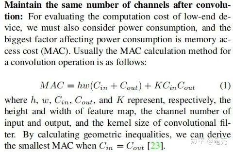
MAC:内存访问成本
计算方法
方法1-使用thop库
1
2
3
4
5
6
7
8
9
10
11
12
13
14
15
16
17
| '''
code by zzg-2020-05-19
pip install thop
'''
import torch
from thop import profile
from models.yolo_nano import YOLONano
device = torch.device("cpu")
net = YOLONano(num_classes=20, image_size=416)
input = torch.randn(1, 3, 416, 416)
flops, params = profile(net, inputs=(input, ))
print("FLOPs=", str(flops/1e9) +'{}'.format("G"))
print("params=", str(params/1e6)+'{}'.format("M")
|
方法2-使用torchstat库
1
2
3
4
5
6
7
8
| '''
在PyTorch中,可以使用torchstat这个库来查看网络模型的一些信息,包括总的参数量params、MAdd、显卡内存占用量和FLOPs等
pip install torchstat
'''
from torchstat import stat
from torchvision.models import resnet50
model = resnet50()
stat(model, (3, 224, 224))
|
方法3-使用ptflops
https://github.com/sovrasov/flops-counter.pytorch
1
2
3
4
5
6
7
|
from ptflops import get_model_complexity_info
from torchvision.models import resnet50
model = resnet50()
flops, params = get_model_complexity_info(model, (3, 224, 224), as_strings=True, print_per_layer_stat=True)
print('Flops: ' + flops)
print('Params: ' + params)
|
模型推理速度正确计算
需要克服GPU异步执行和GPU预热两个问题,下面例子使用 Efficient-net-b0,在进行任何时间测量之前,我们通过网络运行一些虚拟示例来进行“GPU 预热”。这将自动初始化 GPU 并防止它在我们测量时间时进入省电模式。接下来,我们使用 tr.cuda.event 来测量 GPU 上的时间。在这里使用 torch.cuda.synchronize() 至关重要。这行代码执行主机和设备(即GPU和CPU)之间的同步,因此只有在GPU上运行的进程完成后才会进行时间记录。这克服了不同步执行的问题。
1
2
3
4
5
6
7
8
9
10
11
12
13
14
15
16
17
18
19
20
21
22
23
24
25
| model = EfficientNet.from_pretrained(‘efficientnet-b0’)
device = torch.device(“cuda”)
model.to(device)
dummy_input = torch.randn(1, 3, 224, 224,dtype=torch.float).to(device)
starter, ender = torch.cuda.Event(enable_timing=True), torch.cuda.Event(enable_timing=True)
repetitions = 300
timings=np.zeros((repetitions,1))
for _ in range(10):
_ = model(dummy_input)
with torch.no_grad():
for rep in range(repetitions):
starter.record()
_ = model(dummy_input)
ender.record()
torch.cuda.synchronize()
curr_time = starter.elapsed_time(ender)
timings[rep] = curr_time
mean_syn = np.sum(timings) / repetitions
std_syn = np.std(timings)
mean_fps = 1000. / mean_syn
print(' * Mean@1 {mean_syn:.3f}ms Std@5 {std_syn:.3f}ms FPS@1 {mean_fps:.2f}'.format(mean_syn=mean_syn, std_syn=std_syn, mean_fps=mean_fps))
print(mean_syn)
|
模型吞吐量计算
神经网络的吞吐量定义为网络在单位时间内(例如,一秒)可以处理的最大输入实例数。与涉及单个实例处理的延迟不同,为了实现最大吞吐量,我们希望并行处理尽可能多的实例。有效的并行性显然依赖于数据、模型和设备。因此,为了正确测量吞吐量,我们执行以下两个步骤:(1)我们估计允许最大并行度的最佳批量大小;(2)给定这个最佳批量大小,我们测量网络在一秒钟内可以处理的实例数
要找到最佳批量大小,一个好的经验法则是达到 GPU 对给定数据类型的内存限制。这个大小当然取决于硬件类型和网络的大小。找到这个最大批量大小的最快方法是执行二进制搜索。当时间不重要时,简单的顺序搜索就足够了。为此,我们使用 for 循环将批量大小增加 1,直到达到运行时错误为止,这确定了 GPU 可以处理的最大批量大小,用于我们的神经网络模型及其处理的输入数据。
在找到最佳批量大小后,我们计算实际吞吐量。为此,我们希望处理多个批次(100 个批次就足够了),然后使用以下公式:
(批次数 X 批次大小)/(以秒为单位的总时间)
这个公式给出了我们的网络可以在一秒钟内处理的示例数量。下面的代码提供了一种执行上述计算的简单方法(给定最佳批量大小)
1
2
3
4
5
6
7
8
9
10
11
12
13
14
15
16
17
| model = EfficientNet.from_pretrained(‘efficientnet-b0’)
device = torch.device(“cuda”)
model.to(device)
dummy_input = torch.randn(optimal_batch_size, 3,224,224, dtype=torch.float).to(device)
repetitions=100
total_time = 0
with torch.no_grad():
for rep in range(repetitions):
starter, ender = torch.cuda.Event(enable_timing=True),torch.cuda.Event(enable_timing=True)
starter.record()
_ = model(dummy_input)
ender.record()
torch.cuda.synchronize()
curr_time = starter.elapsed_time(ender)/1000
total_time += curr_time
Throughput = (repetitions*optimal_batch_size)/total_time
print(‘Final Throughput:’,Throughput)
|