转载自 SwinTransformer原理源码解读 - 知乎 (zhihu.com)
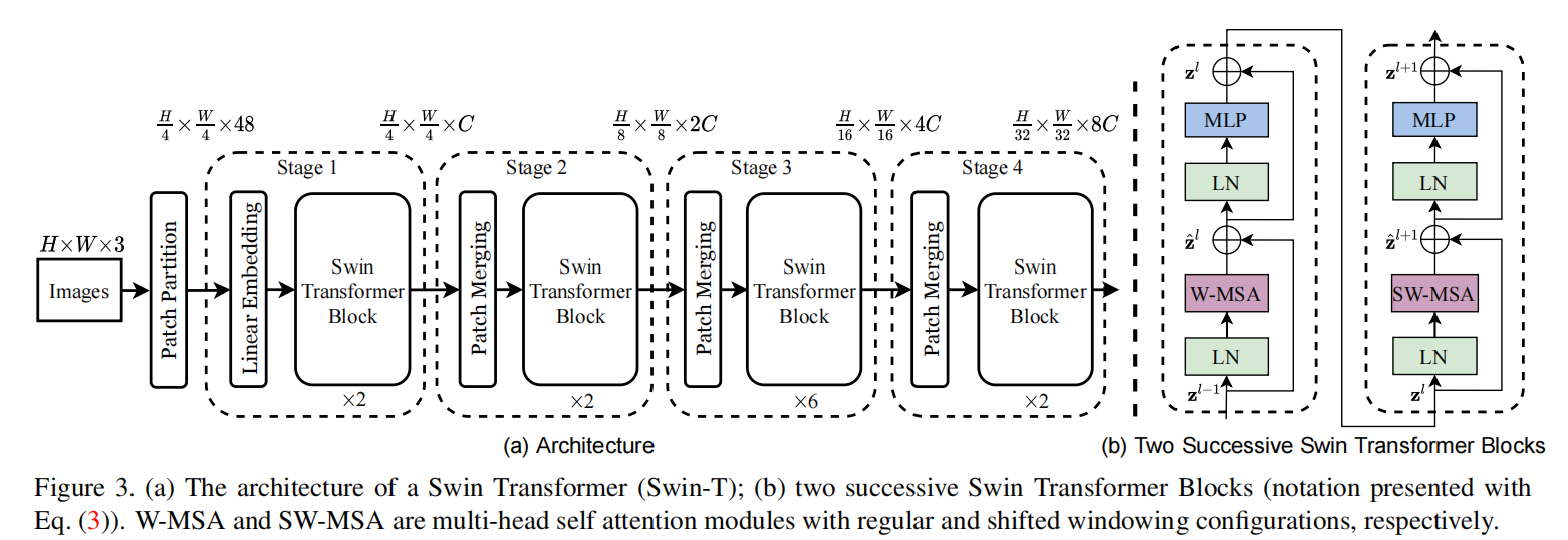
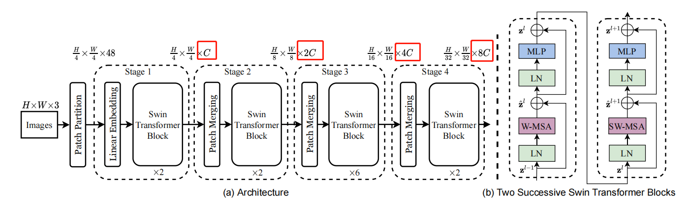
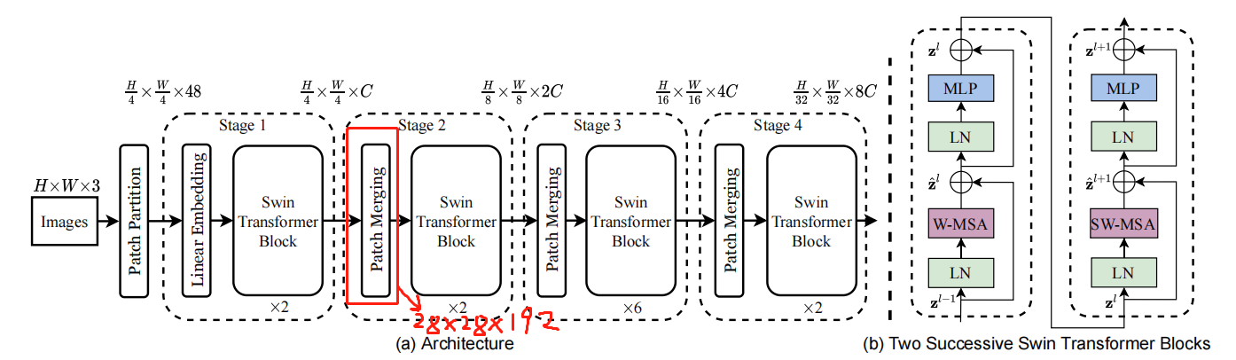
模型总览
如果做分类的话,可以做一个拉直,然后连接分类头即可。
1
2
3
4
5
6
7
8
def forward (self, x ): x = self.features(x) x = self.norm(x) x = x.permute(0 , 3 , 1 , 2 ) x = self.avgpool(x) x = torch.flatten(x, 1 ) x = self.head(x) return x
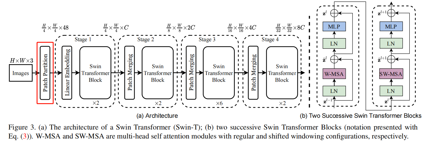
Patch Partition 下面来看Patch Partition的部分
1
2
3
4
5
6
7
8
9
layers.append( nn.Sequential( nn.Conv2d( 3 , embed_dim, kernel_size=(patch_size[0 ], patch_size[1 ]), stride=(patch_size[0 ], patch_size[1 ]) ), Permute([0 , 2 , 3 , 1 ]), norm_layer(embed_dim), ) )
其中,patch_size=[4, 4]
也就是把图片切成56*56个4 * 4 的小patch。
因此,输出为56 *56 * 48。
48 是由 4(patch的H) * 4(patch的W) * 3(patch的深度)算出来的。
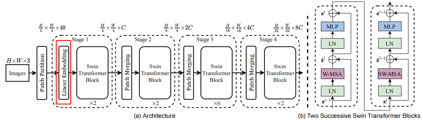
Linear Embedding
对应代码就是上面的,步长=4,卷积核尺寸为4的卷积。
然后,进行Linear Embedding,其中embed_dim=96=C,
接着,使用Permute将输出转换为(B,H,W,C),然后做nn.LayerNorm。nn.LayerNorm的实现及原理
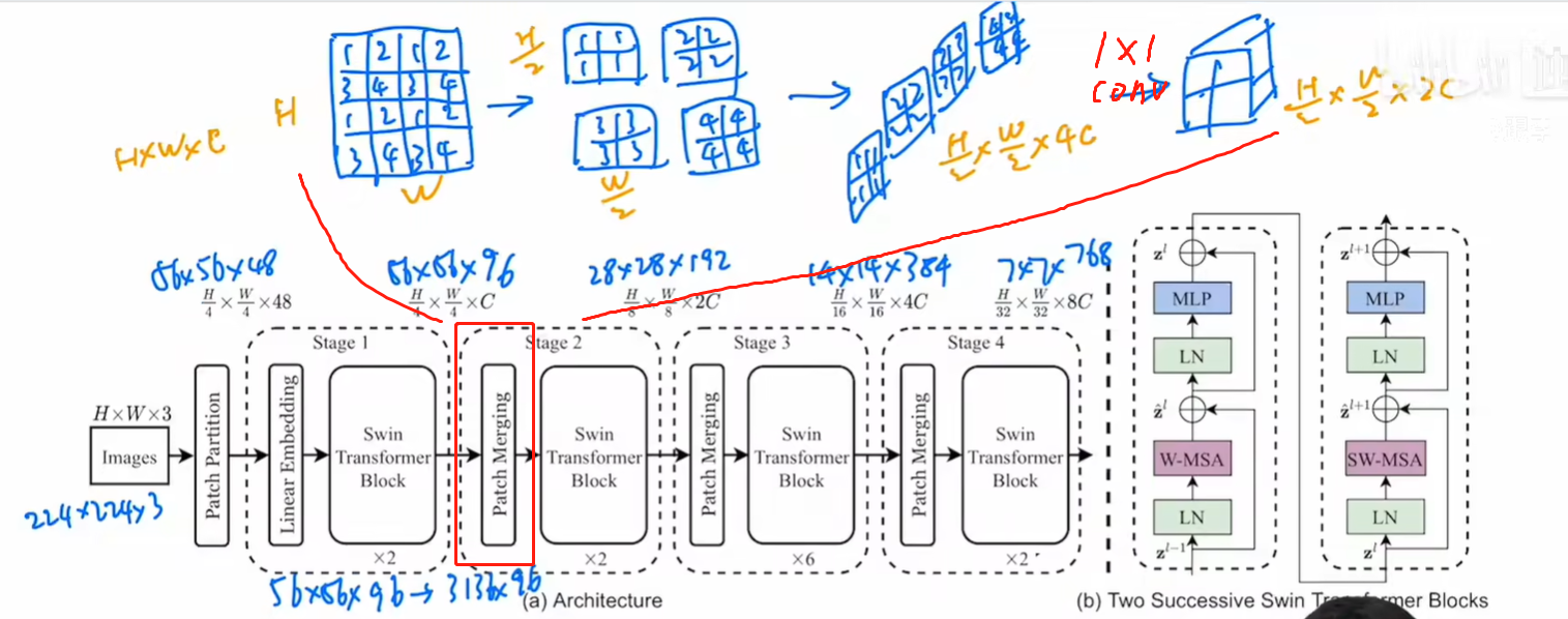
各个stage的维度变化分析 我们来看一下和维度有关的代码
1
2
3
4
5
6
7
8
class SwinTransformer (nn.Module): def __init__ (... ): ... for i_stage in range (len (depths)): dim = embed_dim * 2 ** i_stage for i_layer in range (depths[i_stage]): ...
其中,depths=[2, 2, 6, 2];embed_dim=96=C
由dim = embed_dim * 2 ** i_stage可知,经过每个stage之后的维度变成C、2C、4C、8C
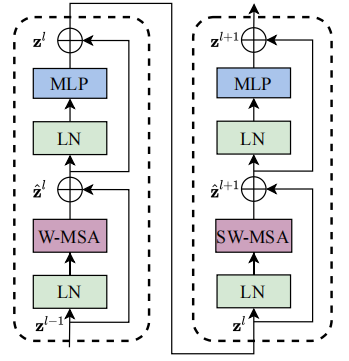
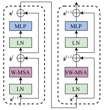
前面已经说了,Block有两种,并且是有前后顺序并同时出现的。
1
2
3
4
5
6
7
8
9
10
11
12
13
14
15
for i_layer in range (depths[i_stage]): ... stage.append( block( dim, num_heads[i_stage], window_size=window_size, shift_size=[0 if i_layer % 2 == 0 else w // 2 for w in window_size], mlp_ratio=mlp_ratio, dropout=dropout, attention_dropout=attention_dropout, stochastic_depth_prob=sd_prob, norm_layer=norm_layer, ) )
其中,window_size=[7, 7]
可以看出,不同之处仅在于shift_size。当i_layer=偶数时,shift_size=[0,0],否则等于[w // 2,w // 2]
下面我们进入block的内部,看看他的定义
1
2
3
4
5
6
7
8
9
10
11
12
13
14
15
16
17
18
19
20
class SwinTransformerBlock (nn.Module): def __init__ (... ): self.norm1 = norm_layer(dim) self.attn = attn_layer( dim, window_size, shift_size, num_heads, attention_dropout=attention_dropout, dropout=dropout, ) self.stochastic_depth = StochasticDepth(stochastic_depth_prob, "row" ) self.norm2 = norm_layer(dim) self.mlp = MLP(dim, [int (dim * mlp_ratio), dim], activation_layer=nn.GELU, inplace=None , dropout=dropout) ... def forward (self, x: Tensor ): x = x + self.stochastic_depth(self.attn(self.norm1(x))) x = x + self.stochastic_depth(self.mlp(self.norm2(x))) return x
LayerNorm
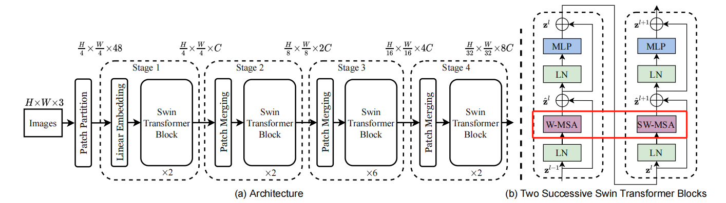
W-MSA或者SW-MSA (W-MSA and SW-MSA are multi-head self attention modules with regular and shifted windowing configurations, respectively.)
stochastic_depth连接
LayerNorm
mlp
stochastic_depth连接
这里面核心的部分就是W-MSA和SW-MSA了,他们定义在ShiftedWindowAttention类中,我们来看看他们做了什么事情。
W-MSA和SW-MSA 1 2 3 4 5 6 7 8 9 10 11 12 13 14 15 16 17 18 19 20 21 22 23 24 25 26 27 28 29 30 31 32 33 34 35 36 37 class ShiftedWindowAttention (nn.Module): def __init__ (... ): ... self.qkv = nn.Linear(dim, dim * 3 , bias=qkv_bias) self.proj = nn.Linear(dim, dim, bias=proj_bias) self.relative_position_bias_table = nn.Parameter( torch.zeros((2 * window_size[0 ] - 1 ) * (2 * window_size[1 ] - 1 ), num_heads) ) coords_h = torch.arange(self.window_size[0 ]) coords_w = torch.arange(self.window_size[1 ]) coords = torch.stack(torch.meshgrid(coords_h, coords_w, indexing="ij" )) coords_flatten = torch.flatten(coords, 1 ) relative_coords = coords_flatten[:, :, None ] - coords_flatten[:, None , :] relative_coords = relative_coords.permute(1 , 2 , 0 ).contiguous() relative_coords[:, :, 0 ] += self.window_size[0 ] - 1 relative_coords[:, :, 1 ] += self.window_size[1 ] - 1 relative_coords[:, :, 0 ] *= 2 * self.window_size[1 ] - 1 relative_position_index = relative_coords.sum (-1 ).view(-1 ) self.register_buffer("relative_position_index" , relative_position_index) nn.init.trunc_normal_(self.relative_position_bias_table, std=0.02 ) def forward (self, x: Tensor ): N = self.window_size[0 ] * self.window_size[1 ] relative_position_bias = self.relative_position_bias_table[self.relative_position_index] relative_position_bias = relative_position_bias.view(N, N, -1 ) relative_position_bias = relative_position_bias.permute(2 , 0 , 1 ).contiguous().unsqueeze(0 ) return shifted_window_attention( ..., shift_size=self.shift_size, ... )
从以上代码可以看出,W-MSA和SW-MSA在定义上几乎一致的,区别仅在于forward()中的shifted_window_attention().
那么,我们就先分析一下他们共性的东西都在做什么事情。
首先是初始化了qkv矩阵、投影矩阵以及相对位置偏差
1
2
3
4
5
6
7
self.qkv = nn.Linear(dim, dim * 3 , bias=qkv_bias) self.proj = nn.Linear(dim, dim, bias=proj_bias) self.relative_position_bias_table = nn.Parameter( torch.zeros((2 * window_size[0 ] - 1 ) * (2 * window_size[1 ] - 1 ), num_heads) )
然后是建立window内的索引
1 2 3 4 5 6 7 8 9 10 11 12 13 14 coords_h = torch.arange(self.window_size[0 ]) coords_w = torch.arange(self.window_size[1 ]) coords = torch.stack(torch.meshgrid(coords_h, coords_w, indexing="ij" )) coords_flatten = torch.flatten(coords, 1 ) relative_coords = coords_flatten[:, :, None ] - coords_flatten[:, None , :] relative_coords = relative_coords.permute(1 , 2 , 0 ).contiguous() relative_coords[:, :, 0 ] += self.window_size[0 ] - 1 relative_coords[:, :, 1 ] += self.window_size[1 ] - 1 relative_coords[:, :, 0 ] *= 2 * self.window_size[1 ] - 1 relative_position_index = relative_coords.sum (-1 ).view(-1 ) self.register_buffer("relative_position_index" , relative_position_index) nn.init.trunc_normal_(self.relative_position_bias_table, std=0.02 )
下面我们看shifted_window_attention:
shifted_window_attention 1 2 3 4 5 6 7 8 9 10 11 12 13 14 15 16 17 18 19 20 21 22 23 24 25 26 27 28 29 30 31 32 33 34 35 36 37 38 39 40 41 42 43 44 45 46 47 48 49 50 51 52 53 54 55 56 57 58 59 60 61 62 63 def shifted_window_attention (... ): B, H, W, C = input .shape pad_r = (window_size[1 ] - W % window_size[1 ]) % window_size[1 ] pad_b = (window_size[0 ] - H % window_size[0 ]) % window_size[0 ] x = F.pad(input , (0 , 0 , 0 , pad_r, 0 , pad_b)) _, pad_H, pad_W, _ = x.shape ... if sum (shift_size) > 0 : x = torch.roll(x, shifts=(-shift_size[0 ], -shift_size[1 ]), dims=(1 , 2 )) num_windows = (pad_H // window_size[0 ]) * (pad_W // window_size[1 ]) x = x.view(B, pad_H // window_size[0 ], window_size[0 ], pad_W // window_size[1 ], window_size[1 ], C) x = x.permute(0 , 1 , 3 , 2 , 4 , 5 ).reshape(B * num_windows, window_size[0 ] * window_size[1 ], C) qkv = F.linear(x, qkv_weight, qkv_bias) qkv = qkv.reshape(x.size(0 ), x.size(1 ), 3 , num_heads, C // num_heads).permute(2 , 0 , 3 , 1 , 4 ) q, k, v = qkv[0 ], qkv[1 ], qkv[2 ] q = q * (C // num_heads) ** -0.5 attn = q.matmul(k.transpose(-2 , -1 )) attn = attn + relative_position_bias if sum (shift_size) > 0 : attn_mask = x.new_zeros((pad_H, pad_W)) h_slices = ((0 , -window_size[0 ]), (-window_size[0 ], -shift_size[0 ]), (-shift_size[0 ], None )) w_slices = ((0 , -window_size[1 ]), (-window_size[1 ], -shift_size[1 ]), (-shift_size[1 ], None )) count = 0 for h in h_slices: for w in w_slices: attn_mask[h[0 ] : h[1 ], w[0 ] : w[1 ]] = count count += 1 attn_mask = attn_mask.view(pad_H // window_size[0 ], window_size[0 ], pad_W // window_size[1 ], window_size[1 ]) attn_mask = attn_mask.permute(0 , 2 , 1 , 3 ).reshape(num_windows, window_size[0 ] * window_size[1 ]) attn_mask = attn_mask.unsqueeze(1 ) - attn_mask.unsqueeze(2 ) attn_mask = attn_mask.masked_fill(attn_mask != 0 , float (-100.0 )).masked_fill(attn_mask == 0 , float (0.0 )) attn = attn.view(x.size(0 ) // num_windows, num_windows, num_heads, x.size(1 ), x.size(1 )) attn = attn + attn_mask.unsqueeze(1 ).unsqueeze(0 ) attn = attn.view(-1 , num_heads, x.size(1 ), x.size(1 )) attn = F.softmax(attn, dim=-1 ) attn = F.dropout(attn, p=attention_dropout) x = attn.matmul(v).transpose(1 , 2 ).reshape(x.size(0 ), x.size(1 ), C) x = F.linear(x, proj_weight, proj_bias) x = F.dropout(x, p=dropout) x = x.view(B, pad_H // window_size[0 ], pad_W // window_size[1 ], window_size[0 ], window_size[1 ], C) x = x.permute(0 , 1 , 3 , 2 , 4 , 5 ).reshape(B, pad_H, pad_W, C) if sum (shift_size) > 0 : x = torch.roll(x, shifts=(shift_size[0 ], shift_size[1 ]), dims=(1 , 2 )) x = x[:, :H, :W, :].contiguous() return x
B, H, W, C = input.shape #数据依次为 32 56 56 96
在第一个block中x.shape和input.shape相同
在W-MSA中,shift_size=[0,0]
partition windows 1 2 num_windows = (pad_H // window_size[0 ]) * (pad_W // window_size[1 ])
其中,pad_H = pad_W = 56;window_size = [7, 7]
因此,特征图会被划分为64块,即 num_windows = 8 * 8 = 64
接下来,对x(维度为(32,56,56,96))执行以下代码:
1 2 x = x.view(B, pad_H // window_size[0 ], window_size[0 ], pad_W // window_size[1 ], window_size[1 ], C) x = x.permute(0 , 1 , 3 , 2 , 4 , 5 ).reshape(B * num_windows, window_size[0 ] * window_size[1 ], C)
第1行会将x的维度转为(32,8,7,8,7,96)。
第2行的permute会将x的维度转为(32,8,8,7,7,96),然后再转为(2048,49,96) # B * nW, Ws * Ws, C。
这么做的目的是并行计算。
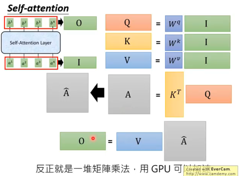
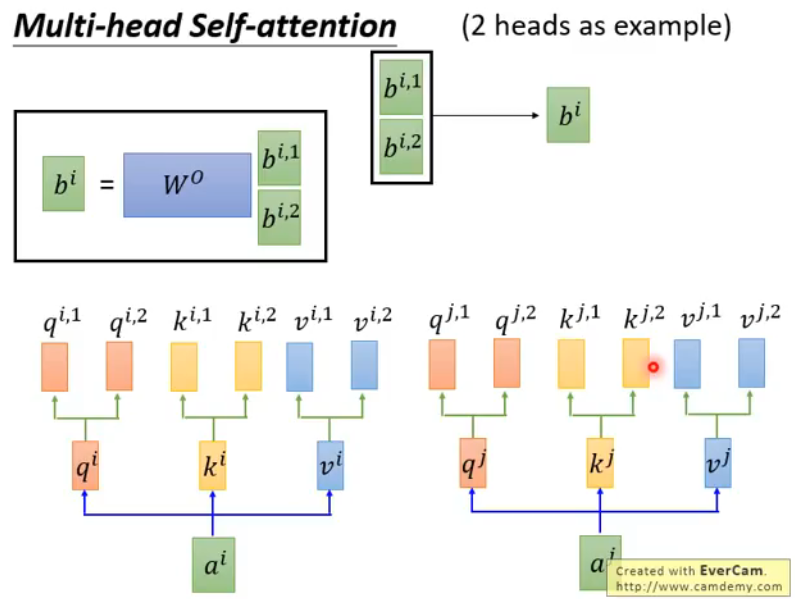
处理完x后,就要进行multi-head attention了。
multi-head attention 1 2 3 4 5 qkv = F.linear(x, qkv_weight, qkv_bias) qkv = qkv.reshape(x.size(0 ), x.size(1 ), 3 , num_heads, C // num_heads).permute(2 , 0 , 3 , 1 , 4 ) q, k, v = qkv[0 ], qkv[1 ], qkv[2 ] q = q * (C // num_heads) ** -0.5 attn = q.matmul(k.transpose(-2 , -1 ))
整个过程可以参考李宏毅的讲义
第2行:qkv.reshape(x.size(0), x.size(1), 3, num_heads, C // num_heads) 得到维度(2048,49,3,3,32)
第3行:q, k, v = qkv[0], qkv[1], qkv[2]
第4行是一种对query做缩放的方式
第5行是query和key求内积。得到的attn的维度是(2048,3,49,49),这里得到49 *49
接下来,对求得的值加上相对位置编码
add relative position bias 1 attn = attn + relative_position_bias
relative_position_bias的维度是(1,3,49,49)
attn归一化和输出结果 1 2 3 4 5 6 attn = F.softmax(attn, dim=-1 ) attn = F.dropout(attn, p=attention_dropout) x = attn.matmul(v).transpose(1 , 2 ).reshape(x.size(0 ), x.size(1 ), C) x = F.linear(x, proj_weight, proj_bias) x = F.dropout(x, p=dropout)
到此,x的维度为(2048,49,96)
关于投射层,就是多头自注意力之后降维到我们想要的维度
下一步要恢复回窗口
reverse windows 1 2 x = x.view(B, pad_H // window_size[0 ], pad_W // window_size[1 ], window_size[0 ], window_size[1 ], C) x = x.permute(0 , 1 , 3 , 2 , 4 , 5 ).reshape(B, pad_H, pad_W, C)
得到的输出维度为(32,56,56,96)
再下一步,进行类似残差连接的操作。
stochastic_depth A LayerNorm (LN) layer is applied
W-MSA小结 以上,我们就完成了W-MSA的过程。W-MSA主要就是在Linear Embedding后的
也就是说,W-MSA在做局部的attention(7 * 7的窗口内做attention)
之所以在局部做attention主要是为了节省计算量,后面我们会量化分析能够节省多少计算
但是在节省计算的同时,也带来了2个问题,第一个就是只能attention到局部的信息,不能attention到更全局的信息,
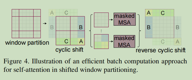
为了解决第二个问题,作者提出了SW-MSA算法(用作者的话The
SW-MSA和W-MSA的区别 先看一下他们在代码上的区别
1 2 3 4 5 6 7 8 9 10 11 12 13 14 15 16 17 18 19 20 21 22 23 24 25 26 27 28 29 30 31 def shifted_window_attention (... ): ... if sum (shift_size) > 0 : x = torch.roll(x, shifts=(-shift_size[0 ], -shift_size[1 ]), dims=(1 , 2 )) ... if sum (shift_size) > 0 : attn_mask = x.new_zeros((pad_H, pad_W)) h_slices = ((0 , -window_size[0 ]), (-window_size[0 ], -shift_size[0 ]), (-shift_size[0 ], None )) w_slices = ((0 , -window_size[1 ]), (-window_size[1 ], -shift_size[1 ]), (-shift_size[1 ], None )) count = 0 for h in h_slices: for w in w_slices: attn_mask[h[0 ] : h[1 ], w[0 ] : w[1 ]] = count count += 1 attn_mask = attn_mask.view(pad_H // window_size[0 ], window_size[0 ], pad_W // window_size[1 ], window_size[1 ]) attn_mask = attn_mask.permute(0 , 2 , 1 , 3 ).reshape(num_windows, window_size[0 ] * window_size[1 ]) attn_mask = attn_mask.unsqueeze(1 ) - attn_mask.unsqueeze(2 ) attn_mask = attn_mask.masked_fill(attn_mask != 0 , float (-100.0 )).masked_fill(attn_mask == 0 , float (0.0 )) attn = attn.view(x.size(0 ) // num_windows, num_windows, num_heads, x.size(1 ), x.size(1 )) attn = attn + attn_mask.unsqueeze(1 ).unsqueeze(0 ) attn = attn.view(-1 , num_heads, x.size(1 ), x.size(1 )) ... if sum (shift_size) > 0 : x = torch.roll(x, shifts=(shift_size[0 ], shift_size[1 ]), dims=(1 , 2 )) ... return x
这个移动窗口采用了一种cyclic shift和 efficient batch computation技巧
Patch Merging 类似于pooling操作,尺寸/2